Understanding the Confusion Matrix

A gentle, story-driven introduction so you’ll never be confused again.

This is Episode 00

The Posts Of The Saga

• Episode 00
• Episode 01
• Episode 02

TL;DR

• For beginners
• We indicate whether the prediction was correct (T/F) + the nature of prediction (P/N)
• FN=Misses, FP=False Alarm
• When the confusion matrix is about X, say aloud:
  • We miss X - <DANGER> => Recall
  • We miss NOT X - <DANGER> => Precision
• Confusion matrix concept extends to multi-class problems

Click the images to zoom in.

Table of Contents

• Introduction
• Drawing The Matrix
• Intuitive Understanding
• The Metrics

Introduction

One day, a great Machine Learning philosopher once whispered to me: “Listen, kid. A Machine Learning project is just like a dish in a fine restaurant. Every step matters, especially the first ones. You can plate it beautifully, serve it with elegance, even impress the critics… but if the recipe is bad, the dish will never be good. And trust me, no amount of fancy deployment can save a rotten model. Capiche?”

Rémy, the ML philosopher

Step	Analogy
EDA	The recipe
Features Engineering	The secret sauce
Baseline model	The first taste
Metrics Analysis	The critics’ score
API & App	Sharing with friends
Deployment & Monitoring	Serve the dish, maintain quality

At one of the very early steps of the process, before jumping into modeling, optimization, and all that fun stuff with Scikit-Learn, it’s absolutely crucial to choose a metric. You also need to be able to explain why you chose it, set yourself a clear goal, and stick to it. And honestly, that’s usually the hardest part. Because when we don’t get the results we want, we all have a tendency to “bend the data” until it says what we want to hear, and that is a very, very bad idea.

When I say “choose a metric,” right away you start hearing words like Recall, Precision, F1-score, Accuracy… On top of that, people start talking about the confusion matrix. And that’s usually where I completely lose my footing.

Let’s be clear. I have no problem with Recall and its friends nor with the formulas in general. No, no, it is even worst than that. The real issue was that for a very long time, I just couldn’t wrap my head around how the labels in the confusion matrix were written: TP, FP, TN, and FN.

Which made it… somewhat awkward to properly explain my choices. But that was before. Since then, I went to Lourdes, I saw the light, and now I almost understand everything.

So yeah, that’s exactly what we’re going to talk about in this post. As usual, I’ll start very slowly, without assuming anything about your math background (okay, you still need to know how to add and divide), but by the end, pinky swear, your ideas will be crystal clear. You’ll be able to choose and explain the metric for your ML project… and also to legitimately worry if a test tells you that you may have caught this or that disease.

Alright. Let’s get started.

Side note

Ancel Keys, the father of the K-ration, is a foundational figure in nutritional epidemiology but remains controversial due to his history of data manipulation. In the 1950s, he presented a correlation between saturated fats and heart disease using only six countries despite having data for 22. This “cherry-picking” tactic was identified as biased as early as 1957 (see Yerushalmy and Hilleboe). Indeed, when the full dataset is considered, the “strong” link Keys claimed largely vanishes.

Any consequence? This skewed “science” (plus a lot of politic) became the foundation for global dietary guidelines, leading the food industry to replace fats with sugar, additives, and ultra-processed ingredients to maintain palatability. This shift has fueled overconsumption and the modern obesity epidemic. By 2025, for the first time in history, childhood obesity rates have overtaken undernutrition globally, signaling a profound crisis in industrial food environments.

So when I say that “bending the data” is a very, very bad idea. I really mean it.

Drawing The Matrix

To kick things off, I want to finally put to rest this whole “how do I draw a confusion matrix?” question.

Let’s imagine we have some “thing” that makes predictions. It could be a ML model, a pregnancy test, a fortune teller… whatever you want, it’s your story.

Now, this binary predictor will sometimes get things right and sometimes get things wrong. If you look closer, you can actually split its predictions into four categories:

1. I said, before going into the club, that I was going to leave with a girl, and sure enough, I left with the one who became my wife (poor thing, for better or for worse, as they say…)
2. I said, before going into the club, that I was going to leave with a girl, but no luck, I went home alone.
3. I said, before going into the club, that I wasn’t going to leave with a girl, and… I went home alone.
4. I said, before going into the club, that I wasn’t going to leave with a girl, but the way I danced to those wild beats… I ended up leaving with the most beautiful girl of the night.

Yeah, I know, the example is silly, but that’s the point, it sticks in your mind. And trust me, when it comes to ridiculous examples, you haven’t seen anything yet. The worst is yet to come…

So, we can sum all this up in a table to evaluate how good the predictions are. If you go clubbing twice a week on average, by the end of the year you’ve made 104 predictions… and now it’s starting to look credible.

Anyway, in the previous paragraph, the key word is “evaluate the accuracy of the predictions”. Yeah, I know, that’s more than one word.

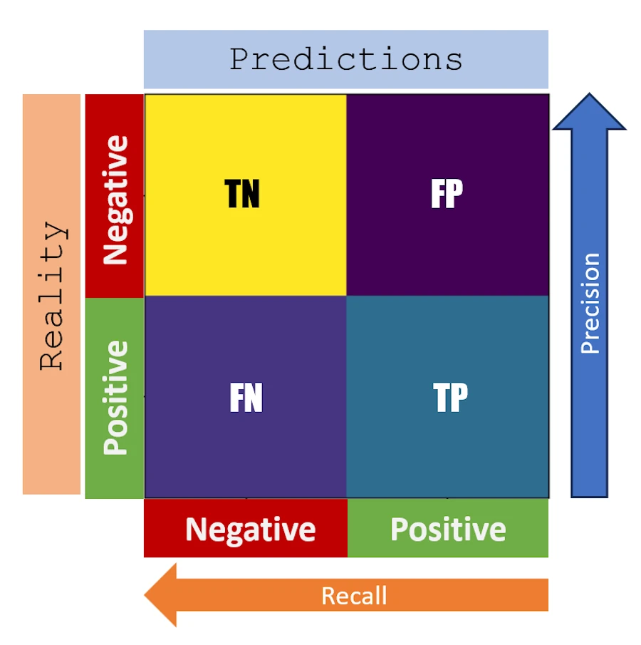
What we’re going to do now is make a two-way table: on one side, you put the predictions, and on the other, you put reality. So it’s a “Reality vs. Predictions” matrix, and for now, don’t worry about which is the row and which is the column.

Now, THE REALLY IMPORTANT THING is that in each cell of the table, we will indicate:

1. whether the prediction was correct
2. AND what kind of prediction it was.

Let’s clarify the vocabulary:

• The prediction is NEGATIVE or POSITIVE. Here, a POSITIVE prediction could mean “I left with a girl”.
• Reality is NEGATIVE or POSITIVE. These are in the same “units” as the predictions so we can compare them.
• The correctness of the prediction compared to reality is TRUE or FALSE.

So I suggest this first empty matrix:

              ┌──────────┬──────────┐
   Negative   │          │          │
REALITY       ├──────────┼──────────┤
   Positive   │          │          │
              └──────────┴──────────┘
                Negative   Positive
                    PREDICTION

Which we will fill in together by announcing what we do “out loud.”

The data: At the end of the year, out of 104 outings, I said I was going to go out with a girl 80 times, but in fact I came home alone 70 times. On the other 24 outings where I said I was going to be serious, I only kept my word 18 times.

Let’s continue, and now I say “loud and clear”:

1. Prediction P and Reality P: bottom right. The prediction is correct. I said that I would meet a girl and that’s what happened (what a charmer!). I write T (the prediction was true) and then P (because the prediction was P). The value is 10 (80–70).

2. Prediction P and Reality N: top right. The prediction is incorrect. I said that I would meet a girl, but I went home alone. I write F (the prediction was false) and then P (because the prediction was P). The value is 70.

3. Prediction N and Reality N: top left. The prediction is correct. I said that I would behave seriously and go home alone, and that is indeed what happened. I write T (the prediction was true) and then N (because the prediction was N). The value is 18.

4. Prediction N and Reality P: bottom left. The prediction is incorrect. I said that I would behave seriously and go home alone, but on those nights I met the girl of my life (at least that’s what I thought at the time). I write F (the prediction was false) and then N (because the prediction was N). The value is 06 (24–18).

Tadaa!

              ┌──────────┬──────────┐
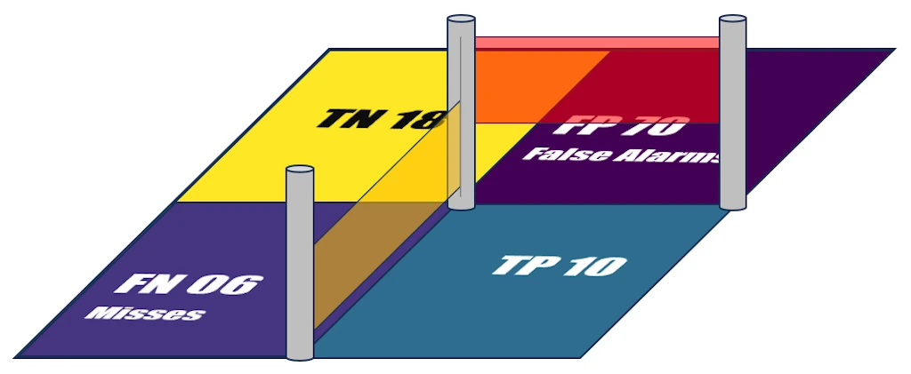
   Negative   │  TN 18   │  FP 70   │
REALITY       ├──────────┼──────────┤
   Positive   │  FN 06   │  TP 10   │
              └──────────┴──────────┘
                Negative   Positive
                    PREDICTION

Notes:

• You can see that it doesn’t really matter what is shown in rows or columns. Here I followed what Scikit-Learn (a library used with Python) displays, but that’s really not the most important part. In this case we have:
  • X-axis (columns): what the model predicted (Negative then Positive)
  • Y-axis (rows): the ground truth (Positive at the bottom, Negative at the top)
• Obviously, the sum of all the cells is 104, the total number of nights out.
• In the same way, with this matrix, the sums of the different columns correspond to my predictions (going home alone 24 times, being a charmer 80 times).
• The sum along the main diagonal (top-left, bottom-right) corresponds to the number of correct predictions (with either positive or negative outcomes, but the predictions were correct: 28).
• The sum along the anti-diagonal (bottom-left, top-right) is the number of times the predictions were wrong (76).

Thins to keep in mind: Each cell contains a two-letter code:

• First letter: whether the prediction was correct (T for True) or wrong (F for False)
• Second letter: the prediction itself (P or N)

Building the Matrix Step by Step

Prediction	Reality	Correct?	Label
P	P	Yes → T	TP
P	N	No → F	FP
N	P	No → F	FN
N	N	Yes → T	TN

Exercices

Exercice 00: Take your cell phone. Now! Set an alarm for next week and the week after and name them “Redraw Confusion Matrix”. The aim is for you to redraw the matrix, label it, and explain out loud (as if you were talking to an invisible friend) what you understand. If it does’nt work as expected, set another alarm in 2 weeks.

Exercise 01: The Martian “To Probe or Not to Probe” Detector. Imagine you are a Martian scout ship commander using a “Human-O-Meter” to decide if a creature on Earth is a Human (Positive) or just a very tall Garden Gnome (Negative). Out of 100 scans:

• Your radar screamed “HUMAN DETECTED!” 60 times. Upon closer inspection, 45 were actual humans, but 15 were just gnomes in trench coats.
• Your radar stayed silent 40 times. However, you later found out that 10 sneaky humans were hiding behind bushes and weren’t detected.
• Task: Draw the confusion matrix and label the TP, FP, TN, and FN counts. Explain to your Martian crew what a “False Alarm” means in this context.

Exercise 02: Batman’s “Joker-Lookalike” Filte.r Batman has a new AI filter for his Bat-Goggles to identify the Joker (Positive) among Gotham’s street performers (Negative).

• In a crowd of 200 people, the filter identified 20 individuals as “The Joker.” In reality, only 2 of them were the real Joker (the other 18 were just really good cosplayers).
• The goggles showed “Harmless Performer” for 180 people. Sadly, the Joker had one more twin brother in that group that the AI missed.
• Task: Build the “Reality vs. Prediction” matrix. If Batman punches a “False Positive,” who is he hitting?

Intuitive Understanding

Before we dive into a bit of algebra, let’s step back and appreciate the matrix we just built. First off, we can be proud of ourselves. More importantly, tomorrow morning you should be able to read it “out loud”, I really mean it, without any trouble. Then, as a bonus challenge, try swapping the rows and columns, or flipping the two rows and/or the two columns around. The results stay the same, only the layout changes. Here, I’m using the format that the excellent Scikit-Learn library uses, but we don’t want our understanding to depend on any particular arrangement.

Speaking of understanding… Let’s try replacing TP and friends with everyday words. Starting from our original matrix:

              ┌──────────┬──────────┐
   Negative   │    TN    │    FP    │
REALITY       ├──────────┼──────────┤
   Positive   │    FN    │    TP    │
              └──────────┴──────────┘
                Negative   Positive
                    PREDICTION

And I propose the following matrix:

              ┌────────────────────┬───────────────┐
   Negative   │ Correct Rejections │  False Alarm  │
REALITY       ├────────────────────┼───────────────┤
   Positive   │      Misses        │      Hits     │
              └────────────────────┴───────────────┘
                      Negative          Positive
                              PREDICTION

1. Hits: Whether it’s at a nightclub, detecting a wildfire on a satellite image, or spotting a fraudulent credit card. You get it. I announced that my natural charisma was going to work its magic once again, and sure enough, I left with a girl. Same thing for wildfire detection and fake cards: we correctly detected what needed to be detected.
2. False Alarm: Okay, the nightclub pickup example doesn’t work great here, but with the wildfire detector, you understand that it screamed “fire!” when there wasn’t one, and we scrambled the water bombers for nothing. Way to go, AI…
3. Correct Rejection: This one’s simple. The fake credit card detector says the card is NOT fraudulent, and that’s indeed the case. As for me, I managed to resist the advances of my many groupies and went home alone (such strength of character, truly inspiring…).
4. Misses: Here, the wildfire detector saw nothing, the credit card detector caught nothing, and I didn’t keep my word. I ended up leaving with a gorgeous young woman even though I’d said I wouldn’t (the willpower of a panda…).

There’s really nothing new here compared to what we’ve already covered, but I think it’s important to be able to put words to math formulas, lines of code, or confusion matrices. It lets you verify that you’ve actually understood, and it confirms that you can explain to a friend what the matrix, formula, or line of code is trying to tell us. Plus, I’m convinced it helps anchor these concepts in our heads.

Alright, let’s do some math. Don’t panic, it’s going to be fine, you’ll see.

Exercices

Exercise 00: The Cursed Treasure Map. You are a treasure hunter with a magical compass that spins when it thinks there is a Treasure Chest (Positive) buried nearby.

• Hit or Miss? The compass spins wildly. You dig and find a chest full of gold. What is the technical term for this?
• False Alarm? The compass spins, you dig for 5 hours, and you only find a dirty old boot. Is this a “Miss” or a “False Alarm”?
• Correct Rejection? You walk over a patch of sand, the compass stays still, and indeed, there is nothing but sand underneath. What label does this get?

Exercise 01: The “She’s Into You” Classifier. You’re at a party and you use an experimental “Crush-Detector” app to see if a girl is “Interested” (Positive) or “Not Interested” (Negative).

• The Heartbreak Miss: The app says “Not Interested,” so you stay in the corner eating chips. Later, you find out she was actually waiting for you to say hi all night. Is this a False Negative or a False Positive?
• The Public Embarrassment: The app flashes “INTERESTED!” You walk up with your best pick-up line about Martians, and she immediately calls security. In the language of the matrix, what just happened?

The Metrics

We’ve mastered the confusion matrix and we understand the “story” it tells us. That’s great, but there’s a small problem. There’s still too much information. How are you going to walk up to your favorite CFO and ask for an extra 2 million dollars in new GPUs because the numbers in your matrix aren’t looking great? That’s not going to fly. Plus, as I mentioned earlier, at the start of any ML project you need to pick one metric and stick with it. A confusion matrix isn’t a metric, it’s a table with 4 numbers. So yeah, that’s not going to work…

In what follows, I’ll use our confusion matrix, which looks like this:

              ┌──────────┬──────────┐
   Negative   │    TN    │    FP    │
REALITY       ├──────────┼──────────┤
   Positive   │    FN    │    TP    │
              └──────────┴──────────┘
                Negative   Positive
                    PREDICTION

Precision

\[\text{Precision} = \frac{\text{TP}}{\text{TP} + \text{FP}}\]

• What matters to us is the number of hits (TP)
• We start with TP, put your index on it in the matrix
• In the last column, we compare TP to the sum of that column
• Storytelling: “Among everything I predicted as Positive, how many were actually Positive?”

Side Note

I just said: “we compare TP to the sum of that column”. I hope it is clear that in order to compare 2 values it is better to divide one by the other than to subtract one by the other. In addition remember we are more sensitive to the proportion than to the absolute magnitudes. See the law of Weber if needed.

Recall

\[\text{Recall} = \frac{\text{TP}}{\text{TP} + \text{FN}}\]

• What matters to us is the number of hits (TP)
• We start with TP
• In the bottom row, we compare TP to the sum of that row
• Storytelling: “Among all actual Positives, how many did I find?”
• The term Recall comes from the field of information retrieval. Out of all the relevant documents available in the database, how many did I retrieve?
• For example, we might want to extract all documents of interest, even if that means pulling a few irrelevant ones along the way.

If this help, we can also picture the situation in 3D. In a perfect world, all my predictions would have been correct and I would have gone out 80 times with girls over the year (TP = 80). But in reality, it’s more like there are sliding doors that are more or less open, and by the end of the year only 10 dates are left.

Out of the 80 dates announced at the beginning, some, not all, leaked into the FP bucket (false alarms), and others slipped under the yellow door and ended up in the FN bucket (misses). I can’t be definitive about these leaks, because FP and FN also contain predictions that originally came from TN.

That said, since there are more elements in FP than in FN, we can reasonably assume that the space under the red door is larger than the one under the yellow door… but hey, that’s still just an assumption.

Confusion Matrix in 3D

F1-score

\[\text{F1-score} = \frac{2}{\frac{1}{\text{Precision}} + \frac{1}{\text{Recall}}}\]

• The F1-score is the harmonic mean of Precision and Recall
• The F1-score looks for a compromise between Precision and Recall
• Storytelling: “How well am I balancing finding all the positives with not crying wolf?”

Let’s go back to the nightclub. I could adopt two extreme strategies:

1. The overconfident guy: Every single night, I announce “Tonight, I’m leaving with someone!” This way, I never miss an opportunity (if there’s a chance). I’ve predicted it (Recall = 100%). But my hit rate is abysmal because most nights I go home alone despite my bold claims (Precision in the gutter).

2. The overcautious guy: I only predict success when I’m absolutely certain (say, when a girl has already shared her phone number while we were queuing outside the nightclub). Sure, when I make a prediction, I’m almost always right (Precision ≈ 100%). But I miss tons of opportunities I didn’t dare call (Recall in the gutter).

The F1-score tells us “Pick a lane, buddy, but not an extreme one.” It forces us to find a balance. And here’s the key property of the harmonic mean: it punishes imbalance harshly. If one metric is great but the other is terrible, the F1-score stays low. You can’t hide a weakness by excelling elsewhere.

If you remember your physics classes, the harmonic mean shows up in two classic situations:

1. Two resistors in parallel

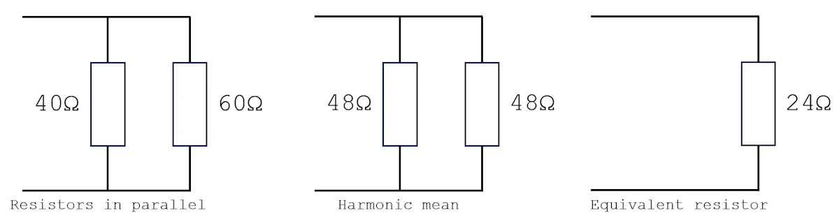
1. A car traveling the same distance at two different speeds

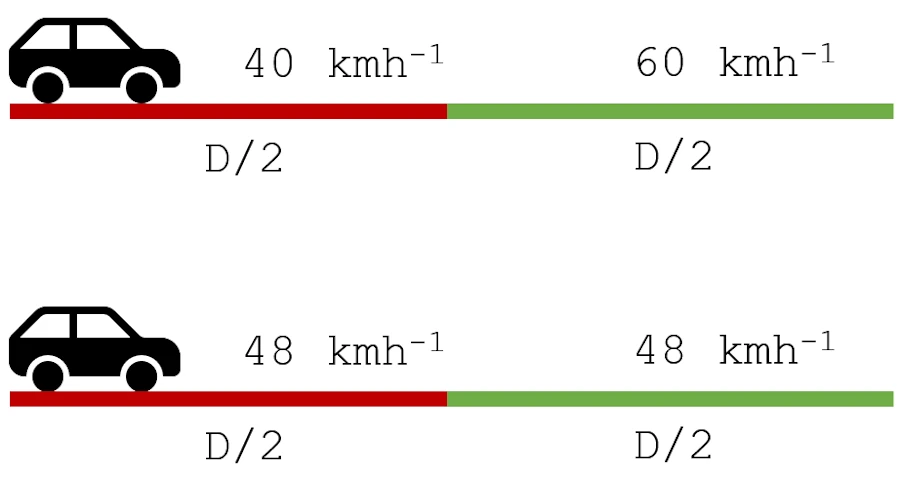
In both cases, we can’t just average the values. Indeed, the smaller one “drags down” the result. Same thing here: a fantastic Precision can’t compensate for a catastrophic Recall, and vice versa.

Accuracy

\[\text{Accuracy} = \frac{\text{TP} + \text{TN}}{\text{Total}}\]

• What “matters” for us, is the number of good predictions (TN+TP)
• First Diagonal over the Total
• Storytelling: “The Accuracy of a predictor is the percentage of correct predictions among all predictions made.”

At this point, it is important to make the distinction between Accuracy and Precision

Accuracy & Precision

Indeed, you can have low accuracy even with a high Precision. See the top-left example below:

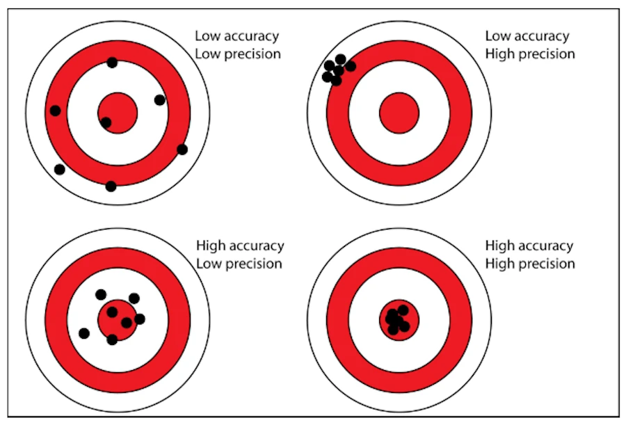
Finally (CeCe Peniston, ‘91) you may want to keep in mind the figure below:

Tadaa!

Confusion Matrix Labels in a Tree

Do you remember when you were young and innocent (MJ, ‘92, Remember the Time). You start learning probabilities and you used to draw trees to simulate, for example, that you toss a coin twice and get 4 possible results (HH, HT, TH, TT).

You know what? We can find the Confusion Matrix labels in the tree you used to draw. See below:

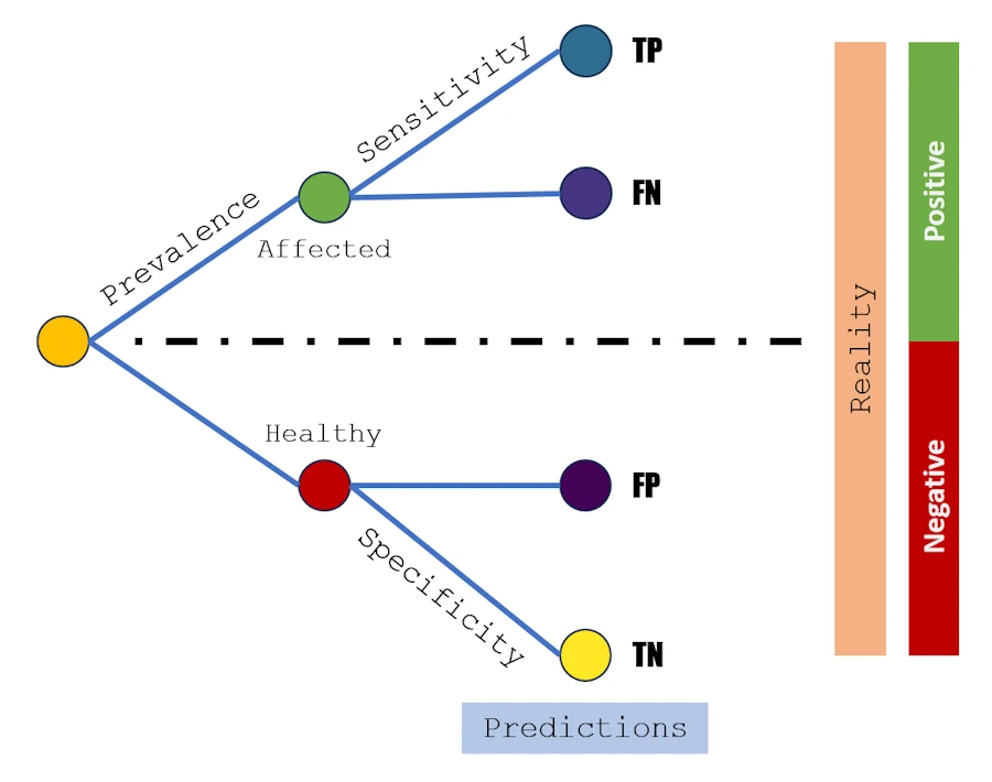
Confusion Matrix metrics in a Tree

We assume that the probability of being sick, called the Prevalence, is a certain percentage of the population. Each person is therefore either sick or healthy.

Then, everyone takes a medical test that has two key characteristics:

• Sensitivity, which is the percentage of sick people who are correctly identified as sick by the test.
• Specificity, which is the percentage of healthy people who are correctly identified as not sick by the test.

Look, at the end of the top branch of the tree for example. We found our friend TP. Indeed, the guy is affected, so the reality is POSITIVE. Then the prediction is “he is affected”, “he is POSITIVE”. So, in this case, the prediction is correct, it is TRUE and so the leaf is labeled TRUE-POSITIVE, aka TP.

Check for yourself but the same reasoning applied to the three other branches and you get: FN, FP and TN.

Now, if we stay focused on the top branch, you may recall that our teacher mentioned the “probability of testing positive given that the patient is sick”. Does the term “conditional probability” ring a bell? No? What about “Bayesian statistics”, often described as the statistics of causes?

While this is not the main topic here, it is worth noting that TP and its friends appear not only in this type of binary tree, but also play a central role in Bayesian statistics.

Exercices

Exercice 00: Draw the same kind of binary tree but in the case of me and my friends clubbing. Calculate Prevalence, Sensitivity and Specificity in percentage using the numbers of the table below.

              ┌──────────┬──────────┐
   Negative   │  TN 18   │  FP 70   │
REALITY       ├──────────┼──────────┤
   Positive   │  FN 06   │  TP 10   │
              └──────────┴──────────┘
                Negative   Positive
                    PREDICTION

Exercise 01: The Monster-Under-The-Bed Security System. You are building a security system for kids to detect Monsters (Positive).

• If your priority is that no child ever wakes up to a monster (meaning you want ZERO Misses), which metric should you maximize: Recall or Precision?
• If parents are complaining because the alarm goes off every time a cat walks by (too many False Alarms), which metric needs to be improved?

Exercise 02: The Batman “F1-Score” Dilemma. Batman is evaluating two Bat-Computer algorithms to catch Catwoman.

• Algorithm A has a Precision of 0.9 (when it says it’s her, it’s almost always her) but a Recall of 0.1 (it misses her 90% of the time).
• Algorithm B has a Precision of 0.5 and a Recall of 0.5.
• Task: Calculate the F1-score for both. Why does the F1-score “punish” Algorithm A so severely? What does this tell Batman about his “calibration”?

The Posts Of The Saga

• Episode 00
• Episode 01
• Episode 02