Understanding the Confusion Matrix

A gentle, story-driven introduction so you’ll never be confused again.

This is Episode 01

The Posts Of The Saga

• Episode 00
• Episode 01
• Episode 02

Click the images to zoom in.

Table of Contents

• The Imbalance Problem
• Confusion Matrix in Code

The Imbalance Problem

One of the most critical and often overlooked issues in machine learning is class imbalance. This problem appears whenever one class is much rarer than the other. Fraud detection is a textbook example.

How rare is fraud, really?

To build intuition, let’s look at real-world orders of magnitude.

• In France, credit card fraud represents about 0.015% of transactions. This means 15 frauds for 100_000 transactions, let’s say roughly 1 for 1_000_000.
• On the other hand, the probability of being struck by lightning in a given year is often quoted around 1 in 1_000_000.

So fraud is exceptionally rare and this rarity is the root cause of many evaluation mistakes.

A simple thought experiment

Assume we have 100_000 transactions.

Fraudulent transactions: \(100{\_}000 \times 0.015\% = 15\) Legitimate transactions: \(100{\_}000 - 15 = 99{\_}985\)

So the dataset looks like this:

Class	Count
Legitimate	99_985
Fraud	15
Total	100_000

The “dummy” predictor

Now consider a very naïve model which predicts “Fraud” 99% of the time, no matter what. This sounds terrible… but let’s play the game and let’s compute its accuracy.

Step 1: Predictions made

Out of 100_000 transactions

• Predicted Fraud: \(99\% \times 100{\_}000 = 99{\_}000\)
• Predicted Legitimate: \(1\% \times 100{\_}000 = 1{\_}000\)

Step 2: Correct predictions

Since only 15 transactions are actually fraud, at most 15 fraud predictions can be correct. All other fraud predictions are false alarms.

Let’s assume the best-case scenario for the dummy model:

• True Positives (Fraud correctly detected): 15
• False Positives (Legitimate flagged as fraud): \(99{\_}000 - 15 = 98{\_}985\)

Now for legitimate predictions:

• True Negatives: at most 1_000 (since there are many legitimate transactions)

The corresponding confusion matrix looks like this:

              ┌────────────┬─────────────┐
   Negative   │  TN 1_000  │  FP 98_985  │
REALITY       ├────────────┼─────────────┤
   Positive   │  FN     0  │  TP     15  │
              └────────────┴─────────────┘
                 Negative      Positive
                       PREDICTION

Step 3: Accuracy calculation

Accuracy is defined as:

\[\text{Accuracy} = \frac{\text{Correct predictions}}{\text{Total predictions}}\]

Correct predictions:

\[15 \text{ (fraud)} + 1{\_}000 \text{ (legitimate)} = 1{\_}015\]

So:

\[\text{Accuracy} = \frac{1{\_}015}{100{\_}000} = 1.015\%\]

This model is almost always wrong, despite predicting fraud constantly.

The Real Trap (the opposite dummy)

Let’s flip the strategy and predict “Legitimate” 100% of the time.

• Correct legitimate predictions: 99_985
• Missed frauds: 15

The corresponding confusion matrix looks like this:

              ┌────────────┬─────────────┐
   Negative   │  TN     0  │  FP      0  │
REALITY       ├────────────┼─────────────┤
   Positive   │  FN    15  │  TP 99_985  │
              └────────────┴─────────────┘
                 Negative      Positive
                       PREDICTION

Accuracy becomes:

\[\text{Accuracy} = \frac{99{\_}985}{100{\_}000} = 99.985\%\]

99.985% accuracy without detecting a single fraud. This is the famous “99% accuracy fraud detector” trap.

Why Accuracy is misleading?

Accuracy answers the question “How often is the model correct overall?”. However with imbalanced datasets, this question is almost meaningless, because:

• The majority class dominates the metric
• A model can ignore the minority class completely and still look “excellent”

In fraud detection, missing fraud is far more costly than mislabeling a legitimate transaction but Accuracy treats all errors equally.

Why do we need Precision and Recall?

To properly evaluate models under imbalance, we need metrics that focus on the rare class:

• Recall (Sensitivity): “Out of all real frauds, how many did we catch?” (do you visualize the bottom line of our matrix in your mind?)
• Precision: “Out of all transactions flagged as fraud, how many were actually fraud?” (do you see the right column?)

These metrics force us to confront the real trade-offs:

• Catching more fraud vs. triggering too many false alarms
• Business cost vs. customer friction

Things to keep in mind

• Is the dataset imbalanced? If yes => Blinking LED 🔴
• In highly imbalanced problems, accuracy can lie

Understanding this helps us to:

• Choose the right metrics to monitor
• Design meaningful models
• Avoiding dangerously misleading conclusions

Exercices

Exercise 00: The Martian Spy Stealth Challenge. Martian spies are very rare. In a city of 1,000,000 people, only 10 are actually Martians.

• If you build a “Lazy Earthling” model that predicts “Not a Martian” for everyone, what will your Accuracy be?
• Why is this “Accuracy” completely useless for the Men In Black?

Exercise 01: Finding the “One Piece” Treasure. There is only 1 “Legendary Treasure” (Positive) in an ocean of 1,000,000 “Empty Barrels” (Negative).

• Your “Treasure Finder 3000” identifies 100 objects as treasure. One of them is the actual Legendary Treasure.
• Task: Compute the Precision. Then, explain why your boss (the Pirate King) cares more about Recall than Accuracy in this specific scenario.

Confusion Matrix in Code

You thought we were in the Matrix? Nah, instead the confusion matrix is in the code. Below you’ll find two complete sample code because I hate partial code you can find in Medium that never works. One is in Python, the other is in Rust. Both use the Titanic dataset.

Python

import pandas as pd
from sklearn.model_selection import train_test_split
from sklearn.impute import SimpleImputer
from sklearn.preprocessing import StandardScaler, OneHotEncoder
from sklearn.compose import ColumnTransformer
from sklearn.linear_model import LogisticRegression
from sklearn.metrics import confusion_matrix, ConfusionMatrixDisplay

# Mandatory when running in a terminal
import matplotlib.pyplot as plt

df = pd.read_csv("data/titanic.csv")
# print("df datatype & shape :", type(df), df.shape)

# In a script one must use print to see the head of dataframe
print("\n\nDataset head:")
print(df.head())

# Remove `PassengerId`, `Name`, `Ticket`, `Cabin` columns from the dataset
df = df.drop(columns=["PassengerId", "Name", "Ticket", "Cabin"])

print("\n\nDataset head (useless col removed) :")
print(df.head())

# ## Preprocessing
# No EDA? What a shame!
# Split the dataset by $X$ and
# $y$ = Survived
# $X$ = Pclass	Sex	Age	SibSp	Parch	Fare	Embarked

y = df.loc[:, "Survived"]

features_list = ["Pclass", "Sex", "Age", "SibSp", "Parch", "Fare", "Embarked"]
X = df.loc[:, features_list]

# Split the data in `train` and `test` sets
X_train, X_test, y_train, y_test = train_test_split(
    # `stratify=y` allows to stratify our sample.
    # Meaning, we will have the same proportion of categories in test and train set
    X,
    y,
    test_size=0.2,
    random_state=0,
    stratify=y,
)

# Deal with missing values with `SimpleImputer`
# Create an imputer for numerical columns
numerical_imputer = SimpleImputer(strategy="mean")

# Apply it on "Age" column.
# ! See the X[["Age"]] to get a 2D array rather than 1D
X_train[["Age"]] = numerical_imputer.fit_transform(X_train[["Age"]])

# In col `Embarked` replace missing val with "Unknown"
categorical_imputer = SimpleImputer(strategy="constant", fill_value="Unknown")
X_train[["Embarked"]] = categorical_imputer.fit_transform(X_train[["Embarked"]])

# Make all the required preprocessing on the train set
print("\n\nX_train head:")
print(X_train.head())

# Reminder, we have : ['Pclass', 'Sex', 'Age', "SibSp", "Parch", "Fare", "Embarked"]
numeric_features = [0, 2, 3, 4, 5]
numeric_transformer = StandardScaler()

categorical_features = [1, 6]
categorical_transformer = OneHotEncoder()

# No change in score with or without drop=first
# TODO: I think it's better without because in `LogisticRegression` there is an l2-type regulation/penalty
# categorical_transformer = OneHotEncoder(drop="first")

# Apply ColumnTransformer to create a pipeline that will apply the above preprocessing
feature_encoder = ColumnTransformer(
    transformers=[
        ("cat", categorical_transformer, categorical_features),
        ("num", numeric_transformer, numeric_features),
    ]
)

X_train = feature_encoder.fit_transform(X_train)
print("\n\nX_train fit_transformed head:")
print(X_train[0:5, :].round(2))  # print first 5 rows (not using iloc since now X_train became a numpy array)

# Build the Logistic Regression model
classifier = LogisticRegression(random_state=0)  # Instantiate model
classifier.fit(X_train, y_train)  # Fit model. Ajustement

y_train_pred = classifier.predict(X_train)
print(f"\n\ny_train predictions head: {y_train_pred[0:5]}")

# Evaluate the model but preprocess `X_test` first
X_test[["Age"]] = numerical_imputer.transform(X_test[["Age"]])
X_test[["Embarked"]] = categorical_imputer.transform(X_test[["Embarked"]])
X_test = feature_encoder.transform(X_test)

y_test_pred = classifier.predict(X_test)
print(f"y_test predictions head: {y_test_pred[0:5]}")

# Create the confusion matrix with `plot_confusion_matrix`
cm = confusion_matrix(y_train, y_train_pred, labels=classifier.classes_)
cm_display = ConfusionMatrixDisplay.from_predictions(y_train, y_train_pred)
cm_display.ax_.set_title("Confusion matrix on train set ")

# Mandatory when running in a terminal
plt.show()

print(f"\n\nAccuracy-score on train set : {classifier.score(X_train, y_train):.3f}")

cm = confusion_matrix(y_test, y_test_pred, labels=classifier.classes_)
cm_display = ConfusionMatrixDisplay.from_predictions(y_test, y_test_pred)
cm_display.ax_.set_title("Confusion matrix on test set ")

# Mandatory when running in a terminal
plt.show()

print(f"Accuracy-score on test set : {classifier.score(X_test, y_test):.3f}")

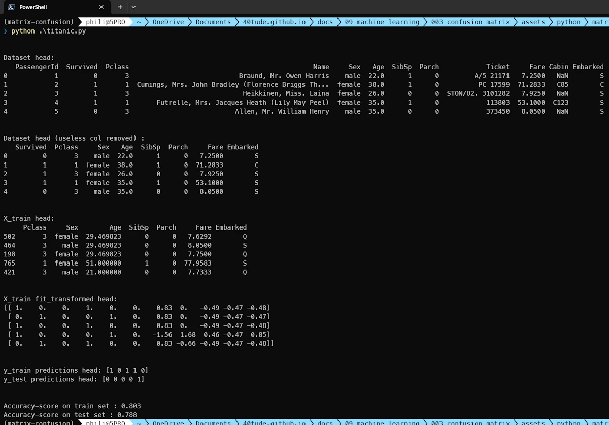
Running the code in the terminal

There is also a Jupyter notebook. The code is the same at 99% and we get the same results.

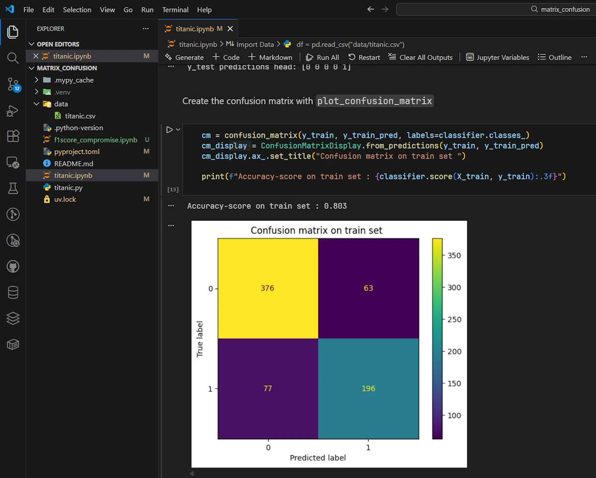
Running the code in VSCode in a Jupyter notebook

So the accuracy is 0.803 on the train set and 0.788 on the test set. Then what?

Good news first. The two values are close which suggests our model isn’t overfitting. It generalizes reasonably well when used with unseen data.

But wait… Should we really be celebrating an 80% accuracy? Well, it depends. Remember what we said earlier: accuracy alone can be misleading. What if 80% of passengers actually died? A dumb model that always predicts “died” would score 80% accuracy without learning anything useful.

Let’s dig deeper and look at the full confusion matrix of the test set (the unseen data).

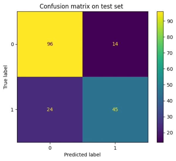
Confusion matrix of the test set

On the screen capture above we can read:

• TN = 96: We correctly predicted 96 passengers would not survive (Correct Rejections)
• FP = 14: We predicted 14 passengers would survive, but they didn’t (False Alarms)
• FN = 24: We predicted 24 passengers wouldn’t survive, but they actually did (Misses)
• TP = 45: We correctly predicted 45 survivors (Hits)

Total: 96 + 14 + 24 + 45 = 179 passengers in the test set (20% of the data set).

Now let’s compute “by hands” our metrics:

• Accuracy = (96 + 45) / 179 = 141 / 179 ≈ 0.788 This matches what sklearn reported
• Precision = 45 / (45 + 14) = 45 / 59 ≈ 0.763 “When I predict survival, I’m right 76% of the time”
• Recall = 45 / (45 + 24) = 45 / 69 ≈ 0.652 “I found 65% of the actual survivors”
• F1-score = 2 × (0.763 × 0.652) / (0.763 + 0.652) ≈ 0.703

What does this tell us? Our model is more cautious than aggressive. It’s better at not crying wolf (decent Precision) than at finding all survivors (lower Recall). In other words, when it predicts someone will survive, it’s fairly reliable. But it misses about a third of the actual survivors.

Is that a problem? It depends on the context and this brings us to our next sections…

Rust

The code below is much longer because

1. I wanted to make sure it “looks like” the code written in Python: imputer, one hot encoding, split test and train datasets…
2. In Python, Scikit-Learn is doing all the hard work for us

// Rust guideline compliant 2025-12-15

use csv::Reader;
use linfa::prelude::*;
use linfa_logistic::LogisticRegression;
use ndarray::{s, Array1, Array2, Axis};
use serde::Deserialize;

/// Passenger record from Titanic dataset
#[derive(Debug, Deserialize)]
#[allow(dead_code)]
struct Passenger {
    #[serde(rename = "PassengerId")]
    passenger_id: u32,

    #[serde(rename = "Survived")]
    survived: u8,

    #[serde(rename = "Pclass")]
    pclass: u8,

    #[serde(rename = "Name")]
    name: String,

    #[serde(rename = "Sex")]
    sex: String,

    #[serde(rename = "Age")]
    age: Option<f64>,

    #[serde(rename = "SibSp")]
    sibsp: Option<u8>,

    #[serde(rename = "Parch")]
    parch: Option<u8>,

    #[serde(rename = "Ticket")]
    ticket: String,

    #[serde(rename = "Fare")]
    fare: f64,

    #[serde(rename = "Cabin")]
    cabin: Option<String>,

    #[serde(rename = "Embarked")]
    embarked: Option<String>,
}

/// Loads Titanic dataset and returns features matrix X and labels y.
///
/// Features: Pclass, Sex, Age, SibSp, Parch, Fare, Embarked (encoded)
///
/// This function mimics the Python preprocessing:
/// - Drops PassengerId, Name, Ticket, Cabin columns
/// - Keeps rows with missing values (imputation done separately)
fn load_titanic(path: &str) -> (Vec<Passenger>, Array1<u8>) {
    let mut rdr = Reader::from_path(path).expect("Failed to read CSV file");

    let mut passengers = Vec::new();
    let mut labels = Vec::new();

    for result in rdr.deserialize::<Passenger>() {
        let p = result.expect("Failed to deserialize passenger");
        labels.push(p.survived);
        passengers.push(p);
    }

    let y = Array1::from(labels);
    (passengers, y)
}

/// Computes mean of non-missing Age values.
fn compute_age_mean(passengers: &[Passenger]) -> f64 {
    let ages: Vec<f64> = passengers.iter().filter_map(|p| p.age).collect();
    let sum: f64 = ages.iter().sum();
    sum / ages.len() as f64
}

/// Imputes missing Age values with mean and missing Embarked with "Unknown".
fn impute_missing(passengers: &mut [Passenger], age_mean: f64) {
    for p in passengers.iter_mut() {
        if p.age.is_none() {
            p.age = Some(age_mean);
        }
        if p.sibsp.is_none() {
            p.sibsp = Some(0);
        }
        if p.parch.is_none() {
            p.parch = Some(0);
        }
        if p.embarked.is_none() {
            p.embarked = Some(String::from("Unknown"));
        }
    }
}

/// One-hot encodes categorical variable.
///
/// Returns (encoded_features, categories) where categories maps index to category name.
fn one_hot_encode(values: &[String]) -> (Array2<f64>, Vec<String>) {
    let mut categories: Vec<String> = values.iter().cloned().collect();
    categories.sort();
    categories.dedup();

    let n_samples = values.len();
    let n_categories = categories.len();
    let mut encoded = Array2::zeros((n_samples, n_categories));

    for (i, val) in values.iter().enumerate() {
        let cat_idx = categories.iter().position(|c| c == val).unwrap();
        encoded[[i, cat_idx]] = 1.0;
    }

    (encoded, categories)
}

/// Converts passengers to feature matrix with preprocessing.
///
/// Features order: Pclass, Sex (one-hot), Age, SibSp, Parch, Fare, Embarked (one-hot)
fn passengers_to_features(passengers: &[Passenger]) -> Array2<f64> {
    // Extract categorical features
    let sex_values: Vec<String> = passengers.iter().map(|p| p.sex.clone()).collect();
    let embarked_values: Vec<String> = passengers
        .iter()
        .map(|p| {
            p.embarked
                .clone()
                .unwrap_or_else(|| String::from("Unknown"))
        })
        .collect();

    // One-hot encode
    let (sex_encoded, _) = one_hot_encode(&sex_values);
    let (embarked_encoded, _) = one_hot_encode(&embarked_values);

    // Extract numeric features
    let n_samples = passengers.len();
    let mut numeric_features = Array2::zeros((n_samples, 5)); // Pclass, Age, SibSp, Parch, Fare

    for (i, p) in passengers.iter().enumerate() {
        numeric_features[[i, 0]] = f64::from(p.pclass);
        numeric_features[[i, 1]] = p.age.unwrap_or(0.0);
        numeric_features[[i, 2]] = f64::from(p.sibsp.unwrap_or(0));
        numeric_features[[i, 3]] = f64::from(p.parch.unwrap_or(0));
        numeric_features[[i, 4]] = p.fare;
    }

    // Concatenate: Sex (one-hot) + numeric + Embarked (one-hot)
    // This matches Python's ColumnTransformer order: cat, num
    let mut features = Array2::zeros((
        n_samples,
        sex_encoded.ncols() + numeric_features.ncols() + embarked_encoded.ncols(),
    ));

    let mut col_idx = 0;

    // Add sex one-hot
    for col in 0..sex_encoded.ncols() {
        features
            .slice_mut(s![.., col_idx])
            .assign(&sex_encoded.column(col));
        col_idx += 1;
    }

    // Add embarked one-hot
    for col in 0..embarked_encoded.ncols() {
        features
            .slice_mut(s![.., col_idx])
            .assign(&embarked_encoded.column(col));
        col_idx += 1;
    }

    // Add numeric features
    for col in 0..numeric_features.ncols() {
        features
            .slice_mut(s![.., col_idx])
            .assign(&numeric_features.column(col));
        col_idx += 1;
    }

    features
}

/// Standardizes features (zero mean, unit variance).
///
/// Returns (standardized_features, mean, std) for later use on test set.
fn standardize_features(x: &Array2<f64>) -> (Array2<f64>, Array1<f64>, Array1<f64>) {
    let mean = x.mean_axis(Axis(0)).unwrap();
    let std = x.std_axis(Axis(0), 0.0);

    let mut x_scaled = x.clone();
    for i in 0..x.ncols() {
        let std_val = if std[i] > 1e-10 { std[i] } else { 1.0 };
        x_scaled
            .column_mut(i)
            .mapv_inplace(|v| (v - mean[i]) / std_val);
    }

    (x_scaled, mean, std)
}

/// Applies standardization using pre-computed mean and std.
fn apply_standardization(x: &Array2<f64>, mean: &Array1<f64>, std: &Array1<f64>) -> Array2<f64> {
    let mut x_scaled = x.clone();
    for i in 0..x.ncols() {
        let std_val = if std[i] > 1e-10 { std[i] } else { 1.0 };
        x_scaled
            .column_mut(i)
            .mapv_inplace(|v| (v - mean[i]) / std_val);
    }
    x_scaled
}

/// Splits data into train and test sets.
///
/// Uses simple 80/20 split (random_state=0 equivalent: first 80% train, last 20% test).
fn train_test_split<T: Clone>(
    x: Array2<f64>,
    y: Array1<T>,
    test_size: f64,
) -> (Array2<f64>, Array2<f64>, Array1<T>, Array1<T>) {
    let n_samples = x.nrows();
    let n_test = (n_samples as f64 * test_size).round() as usize;
    let n_train = n_samples - n_test;

    let x_train = x.slice(s![0..n_train, ..]).to_owned();
    let x_test = x.slice(s![n_train.., ..]).to_owned();
    let y_train = y.slice(s![0..n_train]).to_owned();
    let y_test = y.slice(s![n_train..]).to_owned();

    (x_train, x_test, y_train, y_test)
}

/// Computes confusion matrix.
///
/// Returns [[TN, FP], [FN, TP]]
fn confusion_matrix(y_true: &Array1<u8>, y_pred: &Array1<u8>) -> [[usize; 2]; 2] {
    let mut cm = [[0usize; 2]; 2];

    for (t, p) in y_true.iter().zip(y_pred.iter()) {
        cm[*t as usize][*p as usize] += 1;
    }

    cm
}

/// Computes accuracy score.
fn accuracy_score(y_true: &Array1<u8>, y_pred: &Array1<u8>) -> f64 {
    let correct = y_true
        .iter()
        .zip(y_pred.iter())
        .filter(|(t, p)| t == p)
        .count();
    correct as f64 / y_true.len() as f64
}

fn main() {
    println!("Loading Titanic dataset...\n");

    // Load dataset
    let (mut passengers, y) = load_titanic("data/titanic.csv");

    println!("Dataset shape: {} passengers\n", passengers.len());
    println!("First 5 passengers (before preprocessing):");
    for (i, p) in passengers.iter().take(5).enumerate() {
        println!("{}: {:?}", i, p);
    }

    // Remove useless columns (already done by not including them in features)
    // Columns removed: PassengerId, Name, Ticket, Cabin

    // Preprocessing: impute missing values
    let age_mean = compute_age_mean(&passengers);
    println!("\n\nAge mean for imputation: {:.2}", age_mean);

    impute_missing(&mut passengers, age_mean);

    // Convert to feature matrix
    let x = passengers_to_features(&passengers);
    println!("\nFeature matrix shape: {:?}", x.dim());
    println!("First 5 rows (after encoding):");
    println!("{:.2}", x.slice(s![0..5, ..]));

    // Split into train and test sets (80/20)
    let (x_train, x_test, y_train, y_test) = train_test_split(x, y, 0.2);

    println!(
        "\n\nTrain set: {} samples, Test set: {} samples",
        x_train.nrows(),
        x_test.nrows()
    );

    // Standardize features (fit on train, apply on test)
    let (x_train_scaled, mean, std) = standardize_features(&x_train);
    let x_test_scaled = apply_standardization(&x_test, &mean, &std);

    println!("\nStandardized train set (first 5 rows):");
    println!("{:.2}", x_train_scaled.slice(s![0..5, ..]));

    // Build and train Logistic Regression model
    println!("\n\nTraining Logistic Regression model...");
    let dataset = Dataset::new(x_train_scaled.clone(), y_train.clone());

    let model = LogisticRegression::default()
        .max_iterations(100)
        .fit(&dataset)
        .expect("Failed to fit model");

    // Predictions on train set
    let y_train_pred = model.predict(&x_train_scaled);
    println!(
        "\nTrain predictions (first 5): {:?}",
        y_train_pred.slice(s![0..5])
    );

    // Confusion matrix on train set
    let cm_train = confusion_matrix(&y_train, &y_train_pred);
    println!("\n\nConfusion Matrix on train set:");
    println!("TN: {}  FP: {}", cm_train[0][0], cm_train[0][1]);
    println!("FN: {}  TP: {}", cm_train[1][0], cm_train[1][1]);

    let acc_train = accuracy_score(&y_train, &y_train_pred);
    println!("Accuracy on train set: {:.3}", acc_train);

    // Predictions on test set
    let y_test_pred = model.predict(&x_test_scaled);
    println!(
        "\n\nTest predictions (first 5): {:?}",
        y_test_pred.slice(s![0..5])
    );

    // Confusion matrix on test set
    let cm_test = confusion_matrix(&y_test, &y_test_pred);
    println!("\nConfusion Matrix on test set:");
    println!("TN: {}  FP: {}", cm_test[0][0], cm_test[0][1]);
    println!("FN: {}  TP: {}", cm_test[1][0], cm_test[1][1]);

    let acc_test = accuracy_score(&y_test, &y_test_pred);
    println!("Accuracy on test set: {:.3}", acc_test);
}

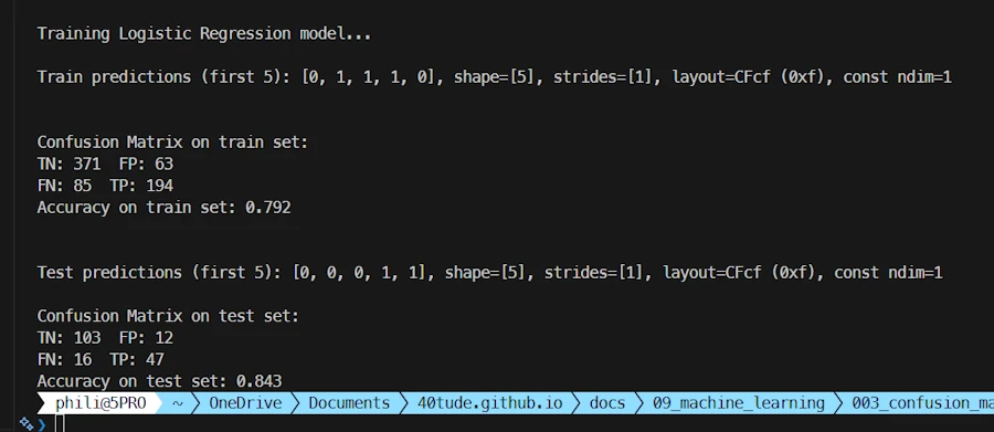
Confusion matrix of the test set

With the Python version we had 0.803 on the train set and 0.788 on the test set. Now we have 0.792 and 0.843. Not so different and to tell the truth I did’nt spend too much time on the differences.

The Posts Of The Saga

• Episode 00
• Episode 01
• Episode 02